3.2.3. Inversion Input File

The inverse problem is solved using the executable program h3dtdinv_v2.exe. The lines of input file are as follows:

Line #	Description	Description
1	Tensor Mesh	path to tensor mesh file
2	Initial Model	initial model
3	Reference Model	reference model
4	Observations File	path to observations file
5	Wave File	sets time steps for the time-dependent problem
6	Active Topography Cells	topography
7	IGNORE	currently ignored by program
8	Bounds	upper and lower bounds for recovered model
9	Weights	additional cell weights
10	beta_max beta_min beta_factor	cooling schedule for beta parameter
11	alpha_s alpha_x alpha_y alpha_z	weighting constants for smallness and smoothness constraints
12	Reference Model Update	reference model update
13	Hard Constraints	use SMOOTH_MOD or SMOOTH_MOD_DIFF
14	Chi Factor	stopping criteria for inversion
15	iter_per_beta tol_ipcg max_iter_ipcg	parameters for Gauss-Newton iterations
16	Solver	choose Pardiso or MUMPS solver
17	Memory Options	store factorizations in RAM or write to disk

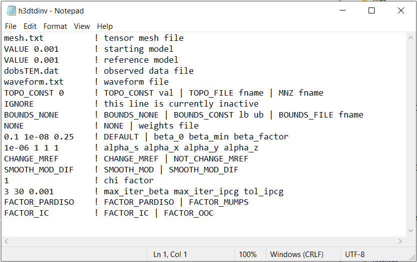
Fig. 3.3 Example input file for the inversion program (Download ).

3.2.3.1. Line Descriptions

• Tensor Mesh: file path to the tensor mesh file

• Initial Model: Defines the starting conductivity model for the inversion. There are two options:

  • FILE filepath: The user enters the flag FILE followed by the path to a conductivity model file

  • VALUE val: The user enters the flag VALUE followed by a value representing the conductivity of all cells lying below the surface topography

• Reference Model: Defines the reference conductivity model for the inversion. There are two options:

  • FILE filepath: The user enters the flag FILE followed by the path to a conductivity model file

  • VALUE val: The user enters the flag VALUE followed by a value representing the conductivity of all cells lying below the surface topography

• Observations File: Set the path to a observations file. The observations file defines the survey geometry, observed data and uncertainties.

• Wave File: Set the path to a wave file. This file defines transmitter current and the time-stepping for the problem.

• Active Topography Cells: Defines the active cells in the inversion. Choices are:

  • TOPO_CONST val: the flag ‘TOPO_CONST’ is followed by an elevation value for the topography

  • TOPO_FILE fname: the flag ‘TOPO_FILE’ is followed by the path to an active cells model

  • MNZ fname: flag ‘MNZ’ is followed by the path to an MNZ file; which contains an N x 3 array denoting the ijk indices of active cells.

• IGNORE: Enter the flag IGNORE. This line is currently not used by the inversion code

• Bounds: Bound constraints on the recovered model. There are 3 options:

  • BOUNDS_NONE: the flag BOUNDS_NONE is provided if there are no bounds on the recovered model

  • BOUNDS_CONST lb ub: the flag BOUNDS_CONST is entered followed by a lower and an upper bound value that will be applied to all cells; e.g. “BOUNDS_CONST 1E-6 0.1”

  • BOUNDS_FILE filepath: the flag BOUNDS_FILE is entered followd by the path to a bounds file

• Weights: Here, the user specifies whether additional weights are supplied. If no additional weights are being supplied, enter the flag NONE. To apply weights, supply the path to a weights file.

• beta_max beta_min beta_factor: Here, the user specifies protocols for the trade-off parameter (beta). beta_max is the initial value of beta, beta_min is the minimum allowable beta the program can use before quitting and beta_factor defines the factor by which beta is decreased at each iteration; example “1E4 10 0.2”. The user may also enter DEFAULT if they wish to have beta calculated automatically.

• alpha_s alpha_x alpha_y alpha_z: Alpha parameters . Here, the user specifies the relative weighting between the smallness and smoothness component penalties on the recovered models.

• Reference Model Update: Here, the user specifies whether the reference model is updated at each inversion step result. If so, enter CHANGE_MREF. If not, enter NOT_CHANGE_MREF.

• Hard Constraints: if the flag SMOOTH_MOD is used, the reference model is not included in the smoothness terms of the model objective function; i.e. we preserve structures in the reference model but not their boundaries. If the flag “SMOOTH_MOD_DIF” is used, the reference model is included in the smallness and smoothness terms of the model objective function; i.e. we preserve the structures and boundaries defined in the reference model. For more, see the GIFtools cookbook .

• Chi Factor: The chi factor defines the target misfit for the inversion. A chi factor of 1 means the target misfit is equal to the total number of data observations.

• iter_per_beta max_iter_ipcg tol_ipcg: Here, iter_per_beta is the number of Gauss-Newton iterations performed for each beta value; see cooling schedule. max_iter_ipcg is the maximum number of iterations for the incomplete-preconditioned-conjugate gradient solve of the Gauss-Newton system, and tol_ipcg defines the tolerance (stopping criteria); see Gauss-Newton solve

• Solver: Define the direct solver that will be used to factor and solve linear systems. Enter one of the following flags:

  • FACTOR_PARDISO: Factor and solve linear systems with Pardiso solver

  • FACTOR_MUMPS: Factor and solve linear systems with MUMPS solver

• Memory Options: Enter one of the following flags:

  • FACTOR_IC: Store factorization in the computer’s RAM. This options is much faster but can only be used on problems of a reasonable size

  • FACTOR_OOC: Writes the factorizations of linear systems to disk. Slower but capable of solving much larger problems.